Case_Study_1
Team Project - Babatunde John Olanipekun, Yvan Sojdehei and Mingyang Nick YU
9/30/2020
Beer App
Beer and Breweries Exploration
Introduction: This is an exploratory data analysis for the data set between Beers.csv and Breweries.csv for CEO and CFO of Budweiser
Loading the datasets
Doing intial inspection of data through various methods below.
# dataset should be in the same folder of this RMD file
Beers = read.csv("/Users/ysojd/Desktop/GRAD SCHOOL COURSEWORK/MSDS_6306_Doing-Data-Science-Master/MSDS_6306_Doing-Data-Science-Master/Unit 8 and 9 Case Study 1/Beers.csv",header = TRUE) #loading beers dataset
Breweries = read.csv("/Users/ysojd/Desktop/GRAD SCHOOL COURSEWORK/MSDS_6306_Doing-Data-Science-Master/MSDS_6306_Doing-Data-Science-Master/Unit 8 and 9 Case Study 1/Breweries.csv",header = TRUE) #loading breweries dataset
#below this line is for self analyzation
#summary(Beers)
#str(Beers)
##Beers$IBU
#summary(Breweries)
#str(Breweries)
#Above this line is for self analyzing can be deleted later
# trim state column
Breweries$State = trimws(Breweries$State)
#Turn Breweries State column into a factor
Breweries$State = as.factor(Breweries$State)
How many breweries are present in each state?
- As we can see by the plot below, each state’s breweries count is displayed in a bar chart
- To make it easier to see which state has the most breweries, we assorted the breweries count by descending order
library(dplyr)##
## Attaching package: 'dplyr'## The following objects are masked from 'package:stats':
##
## filter, lag## The following objects are masked from 'package:base':
##
## intersect, setdiff, setequal, unionlibrary(tidyverse) ## -- Attaching packages --------------------------------------- tidyverse 1.3.0 --## v ggplot2 3.3.2 v purrr 0.3.4
## v tibble 3.0.3 v stringr 1.4.0
## v tidyr 1.1.2 v forcats 0.5.0
## v readr 1.3.1## -- Conflicts ------------------------------------------ tidyverse_conflicts() --
## x dplyr::filter() masks stats::filter()
## x dplyr::lag() masks stats::lag()library(ggplot2)
num_Breweries_by_state <- Breweries %>% group_by(State) %>% dplyr::summarise(count=n())## `summarise()` ungrouping output (override with `.groups` argument)num_Breweries_by_state## # A tibble: 51 x 2
## State count
## <fct> <int>
## 1 AK 7
## 2 AL 3
## 3 AR 2
## 4 AZ 11
## 5 CA 39
## 6 CO 47
## 7 CT 8
## 8 DC 1
## 9 DE 2
## 10 FL 15
## # ... with 41 more rows#As we can see the number of breweries per state is in the list below, to see this better we will use a plot to show results
ggplot(data=num_Breweries_by_state)+
geom_bar(mapping=aes(x=State,y=count,fill=State),stat="identity") +
coord_flip()+
ggtitle("Breweries count by state")+xlab("State")+ylab("Count of Breweries")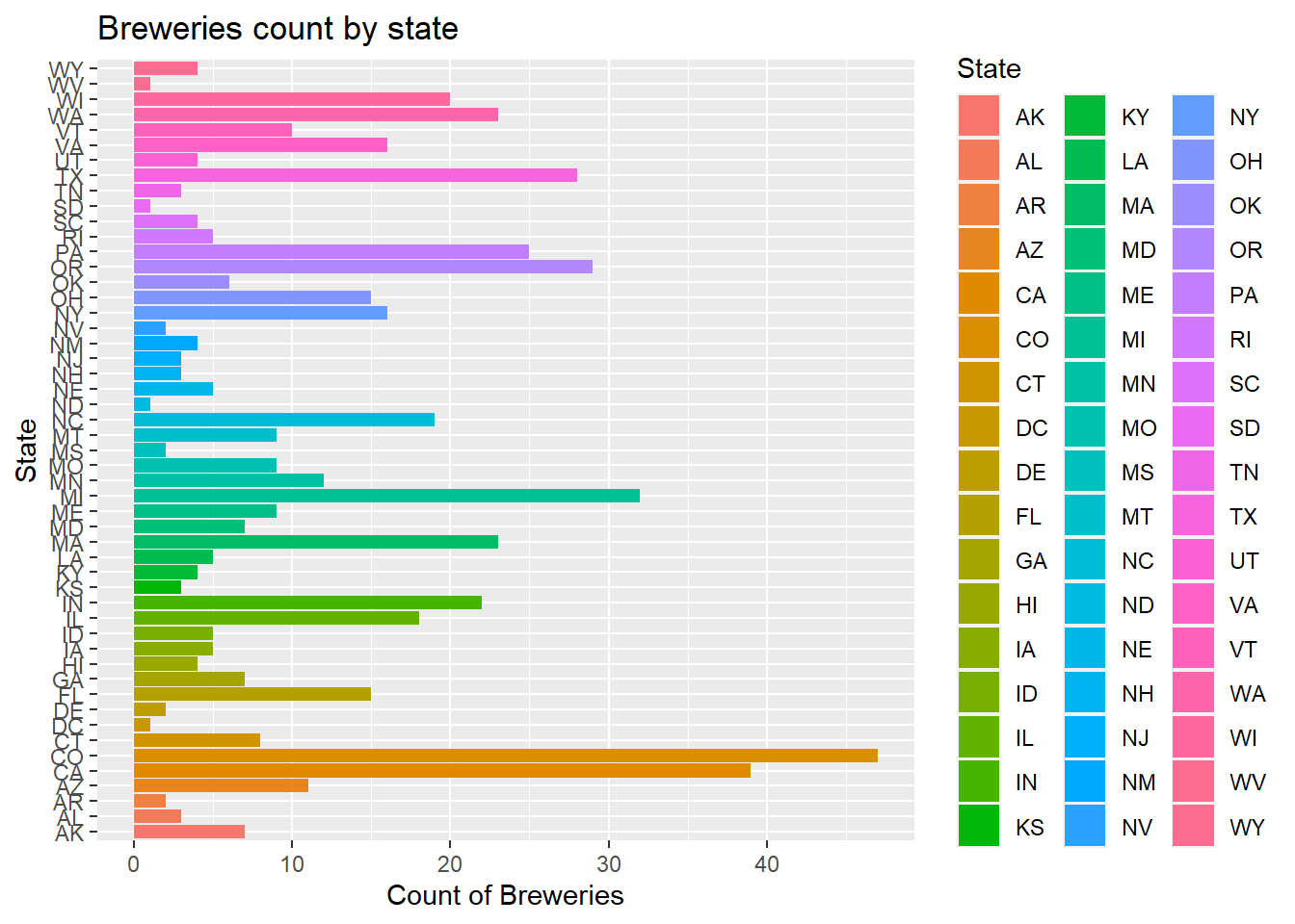
#To see this in order
ggplot(data=num_Breweries_by_state)+
  geom_bar(mapping=aes(x=reorder(State,-count),y=count,fill=State),stat="identity") +
  coord_flip()+
  ggtitle("Breweries count by state")+xlab("State")+ylab("Count of Breweries")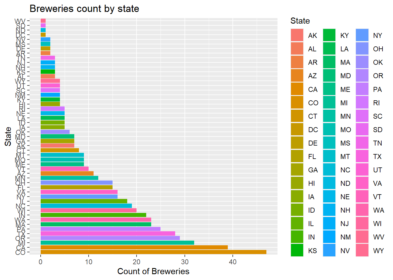
Merge beer data with the breweries data. Print the first 6 observations and the last six observations to check the merged file.
Beers <- Beers %>% dplyr::rename(Brew_ID = Brewery_id)
Beers.with.Breweries = left_join(Beers,Breweries, by = "Brew_ID")
Beers.with.Breweries = Beers.with.Breweries %>% rename(Beer_Name= Name.x)
Beers.with.Breweries = Beers.with.Breweries %>% rename(Brew_Name= Name.y)
head(Beers.with.Breweries,6)
## Beer_Name Beer_ID ABV IBU Brew_ID Style
## 1 Pub Beer 1436 0.050 NA 409 American Pale Lager
## 2 Devil's Cup 2265 0.066 NA 178 American Pale Ale (APA)
## 3 Rise of the Phoenix 2264 0.071 NA 178 American IPA
## 4 Sinister 2263 0.090 NA 178 American Double / Imperial IPA
## 5 Sex and Candy 2262 0.075 NA 178 American IPA
## 6 Black Exodus 2261 0.077 NA 178 Oatmeal Stout
## Ounces Brew_Name City State
## 1 12 10 Barrel Brewing Company Bend OR
## 2 12 18th Street Brewery Gary IN
## 3 12 18th Street Brewery Gary IN
## 4 12 18th Street Brewery Gary IN
## 5 12 18th Street Brewery Gary IN
## 6 12 18th Street Brewery Gary INAddress the missing values in each column
- There are 62 missing values on ABV column, and there are 1005 missing values on IBU column
- Since 1005/2410 is too big of a percentage of missing value for column IBU, I decided to use Predictive mean matching method(widely used statistical imputation method for missing values, first proposed by Donald B. Rubin in 1986 and R. J. A. Little in 1988) to fill the missing data.
- After generating and filling in the missing data, through density plot below, we can see the generated filled in value matches the original density plot. Thus minimize any bias from the researcher of arbitrarily filling in value or overeasily using the overall mean for all missing value
summary(Beers.with.Breweries)## Beer_Name Beer_ID ABV IBU
## Length:2410 Min. : 1.0 Min. :0.00100 Min. : 4.00
## Class :character 1st Qu.: 808.2 1st Qu.:0.05000 1st Qu.: 21.00
## Mode :character Median :1453.5 Median :0.05600 Median : 35.00
## Mean :1431.1 Mean :0.05977 Mean : 42.71
## 3rd Qu.:2075.8 3rd Qu.:0.06700 3rd Qu.: 64.00
## Max. :2692.0 Max. :0.12800 Max. :138.00
## NA's :62 NA's :1005
## Brew_ID Style Ounces Brew_Name
## Min. : 1.0 Length:2410 Min. : 8.40 Length:2410
## 1st Qu.: 94.0 Class :character 1st Qu.:12.00 Class :character
## Median :206.0 Mode :character Median :12.00 Mode :character
## Mean :232.7 Mean :13.59
## 3rd Qu.:367.0 3rd Qu.:16.00
## Max. :558.0 Max. :32.00
##
## City State
## Length:2410 CO : 265
## Class :character CA : 183
## Mode :character MI : 162
## IN : 139
## TX : 130
## OR : 125
## (Other):1406library(mice) #Load mice library to analyze the pattern of missing data##
## Attaching package: 'mice'## The following objects are masked from 'package:base':
##
## cbind, rbindmd.pattern(Beers.with.Breweries)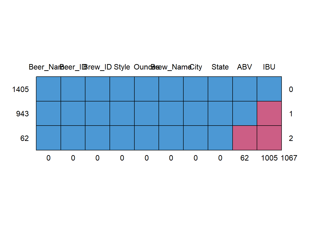
##      Beer_Name Beer_ID Brew_ID Style Ounces Brew_Name City State ABV  IBU
## 1405         1       1       1     1      1         1    1     1   1    1    0
## 943          1       1       1     1      1         1    1     1   1    0    1
## 62           1       1       1     1      1         1    1     1   0    0    2
##              0       0       0     0      0         0    0     0  62 1005 1067
# Since there is large amont of data missing in IBM column
#Try to impute the missing data with Predictive mean Matching method
tempData <- mice(Beers.with.Breweries,m=5,maxit=50,meth='pmm',seed=20)##
## iter imp variable
## 1 1 ABV IBU
## 1 2 ABV IBU
## 1 3 ABV IBU
## 1 4 ABV IBU
## 1 5 ABV IBU
## 2 1 ABV IBU
## 2 2 ABV IBU
## 2 3 ABV IBU
## 2 4 ABV IBU
## 2 5 ABV IBU
## 3 1 ABV IBU
## 3 2 ABV IBU
## 3 3 ABV IBU
## 3 4 ABV IBU
## 3 5 ABV IBU
## 4 1 ABV IBU
## 4 2 ABV IBU
## 4 3 ABV IBU
## 4 4 ABV IBU
## 4 5 ABV IBU
## 5 1 ABV IBU
## 5 2 ABV IBU
## 5 3 ABV IBU
## 5 4 ABV IBU
## 5 5 ABV IBU
## 6 1 ABV IBU
## 6 2 ABV IBU
## 6 3 ABV IBU
## 6 4 ABV IBU
## 6 5 ABV IBU
## 7 1 ABV IBU
## 7 2 ABV IBU
## 7 3 ABV IBU
## 7 4 ABV IBU
## 7 5 ABV IBU
## 8 1 ABV IBU
## 8 2 ABV IBU
## 8 3 ABV IBU
## 8 4 ABV IBU
## 8 5 ABV IBU
## 9 1 ABV IBU
## 9 2 ABV IBU
## 9 3 ABV IBU
## 9 4 ABV IBU
## 9 5 ABV IBU
## 10 1 ABV IBU
## 10 2 ABV IBU
## 10 3 ABV IBU
## 10 4 ABV IBU
## 10 5 ABV IBU
## 11 1 ABV IBU
## 11 2 ABV IBU
## 11 3 ABV IBU
## 11 4 ABV IBU
## 11 5 ABV IBU
## 12 1 ABV IBU
## 12 2 ABV IBU
## 12 3 ABV IBU
## 12 4 ABV IBU
## 12 5 ABV IBU
## 13 1 ABV IBU
## 13 2 ABV IBU
## 13 3 ABV IBU
## 13 4 ABV IBU
## 13 5 ABV IBU
## 14 1 ABV IBU
## 14 2 ABV IBU
## 14 3 ABV IBU
## 14 4 ABV IBU
## 14 5 ABV IBU
## 15 1 ABV IBU
## 15 2 ABV IBU
## 15 3 ABV IBU
## 15 4 ABV IBU
## 15 5 ABV IBU
## 16 1 ABV IBU
## 16 2 ABV IBU
## 16 3 ABV IBU
## 16 4 ABV IBU
## 16 5 ABV IBU
## 17 1 ABV IBU
## 17 2 ABV IBU
## 17 3 ABV IBU
## 17 4 ABV IBU
## 17 5 ABV IBU
## 18 1 ABV IBU
## 18 2 ABV IBU
## 18 3 ABV IBU
## 18 4 ABV IBU
## 18 5 ABV IBU
## 19 1 ABV IBU
## 19 2 ABV IBU
## 19 3 ABV IBU
## 19 4 ABV IBU
## 19 5 ABV IBU
## 20 1 ABV IBU
## 20 2 ABV IBU
## 20 3 ABV IBU
## 20 4 ABV IBU
## 20 5 ABV IBU
## 21 1 ABV IBU
## 21 2 ABV IBU
## 21 3 ABV IBU
## 21 4 ABV IBU
## 21 5 ABV IBU
## 22 1 ABV IBU
## 22 2 ABV IBU
## 22 3 ABV IBU
## 22 4 ABV IBU
## 22 5 ABV IBU
## 23 1 ABV IBU
## 23 2 ABV IBU
## 23 3 ABV IBU
## 23 4 ABV IBU
## 23 5 ABV IBU
## 24 1 ABV IBU
## 24 2 ABV IBU
## 24 3 ABV IBU
## 24 4 ABV IBU
## 24 5 ABV IBU
## 25 1 ABV IBU
## 25 2 ABV IBU
## 25 3 ABV IBU
## 25 4 ABV IBU
## 25 5 ABV IBU
## 26 1 ABV IBU
## 26 2 ABV IBU
## 26 3 ABV IBU
## 26 4 ABV IBU
## 26 5 ABV IBU
## 27 1 ABV IBU
## 27 2 ABV IBU
## 27 3 ABV IBU
## 27 4 ABV IBU
## 27 5 ABV IBU
## 28 1 ABV IBU
## 28 2 ABV IBU
## 28 3 ABV IBU
## 28 4 ABV IBU
## 28 5 ABV IBU
## 29 1 ABV IBU
## 29 2 ABV IBU
## 29 3 ABV IBU
## 29 4 ABV IBU
## 29 5 ABV IBU
## 30 1 ABV IBU
## 30 2 ABV IBU
## 30 3 ABV IBU
## 30 4 ABV IBU
## 30 5 ABV IBU
## 31 1 ABV IBU
## 31 2 ABV IBU
## 31 3 ABV IBU
## 31 4 ABV IBU
## 31 5 ABV IBU
## 32 1 ABV IBU
## 32 2 ABV IBU
## 32 3 ABV IBU
## 32 4 ABV IBU
## 32 5 ABV IBU
## 33 1 ABV IBU
## 33 2 ABV IBU
## 33 3 ABV IBU
## 33 4 ABV IBU
## 33 5 ABV IBU
## 34 1 ABV IBU
## 34 2 ABV IBU
## 34 3 ABV IBU
## 34 4 ABV IBU
## 34 5 ABV IBU
## 35 1 ABV IBU
## 35 2 ABV IBU
## 35 3 ABV IBU
## 35 4 ABV IBU
## 35 5 ABV IBU
## 36 1 ABV IBU
## 36 2 ABV IBU
## 36 3 ABV IBU
## 36 4 ABV IBU
## 36 5 ABV IBU
## 37 1 ABV IBU
## 37 2 ABV IBU
## 37 3 ABV IBU
## 37 4 ABV IBU
## 37 5 ABV IBU
## 38 1 ABV IBU
## 38 2 ABV IBU
## 38 3 ABV IBU
## 38 4 ABV IBU
## 38 5 ABV IBU
## 39 1 ABV IBU
## 39 2 ABV IBU
## 39 3 ABV IBU
## 39 4 ABV IBU
## 39 5 ABV IBU
## 40 1 ABV IBU
## 40 2 ABV IBU
## 40 3 ABV IBU
## 40 4 ABV IBU
## 40 5 ABV IBU
## 41 1 ABV IBU
## 41 2 ABV IBU
## 41 3 ABV IBU
## 41 4 ABV IBU
## 41 5 ABV IBU
## 42 1 ABV IBU
## 42 2 ABV IBU
## 42 3 ABV IBU
## 42 4 ABV IBU
## 42 5 ABV IBU
## 43 1 ABV IBU
## 43 2 ABV IBU
## 43 3 ABV IBU
## 43 4 ABV IBU
## 43 5 ABV IBU
## 44 1 ABV IBU
## 44 2 ABV IBU
## 44 3 ABV IBU
## 44 4 ABV IBU
## 44 5 ABV IBU
## 45 1 ABV IBU
## 45 2 ABV IBU
## 45 3 ABV IBU
## 45 4 ABV IBU
## 45 5 ABV IBU
## 46 1 ABV IBU
## 46 2 ABV IBU
## 46 3 ABV IBU
## 46 4 ABV IBU
## 46 5 ABV IBU
## 47 1 ABV IBU
## 47 2 ABV IBU
## 47 3 ABV IBU
## 47 4 ABV IBU
## 47 5 ABV IBU
## 48 1 ABV IBU
## 48 2 ABV IBU
## 48 3 ABV IBU
## 48 4 ABV IBU
## 48 5 ABV IBU
## 49 1 ABV IBU
## 49 2 ABV IBU
## 49 3 ABV IBU
## 49 4 ABV IBU
## 49 5 ABV IBU
## 50 1 ABV IBU
## 50 2 ABV IBU
## 50 3 ABV IBU
## 50 4 ABV IBU
## 50 5 ABV IBU#summary(tempData)
# completed dataset after adding in generated predictive values
completedData <- complete(tempData,1)
#head(completedData)
# Density plot original vs imputed dataset
densityplot(tempData)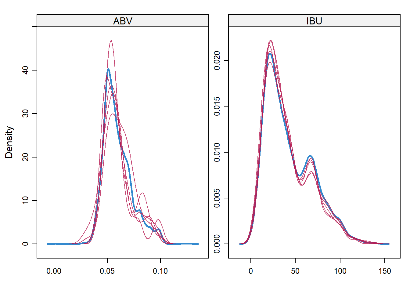
#Note: idea used above to impute data is from link below:
#https://datascienceplus.com/imputing-missing-data-with-r-mice-package/
Compute the median alcohol content and international bitterness unit for each state. Plot a bar chart to compare
- First plotted Median alcohol content by state, one with modified data set, and the other one with non-modified data set
- Then plotted Median international bitterness unit for each state, both on the modified data set and non-modified
- We can see between the modified data and non-modified data provides very different answers. If possible, going back to try to complete the missing data will make the graphics more accurate. But this is a random estimate of the actual value
#Compute and display Median of ABV and IBU by state:
median = completedData %>% group_by(State) %>%
  summarize(median_ABV=median(ABV),median_IBU=median(IBU))
## `summarise()` ungrouping output (override with `.groups` argument)median## # A tibble: 51 x 3
## State median_ABV median_IBU
## <fct> <dbl> <dbl>
## 1 AK 0.056 35
## 2 AL 0.06 39.5
## 3 AR 0.052 72
## 4 AZ 0.055 28
## 5 CA 0.058 36
## 6 CO 0.061 35
## 7 CT 0.06 32
## 8 DC 0.0625 75
## 9 DE 0.0705 52
## 10 FL 0.0555 36.5
## # ... with 41 more rows#Draw Bar Charts to compare
#First plot median of alcohol content using modified data
median %>% ggplot()+
geom_bar(mapping=aes(x=reorder(State,-median_ABV),y=median_ABV,fill=State),stat="identity") +
coord_flip()+
ggtitle("Median Alcohol content by State on modified dataset")+xlab("State")+ylab("Alcohol Content Percentage")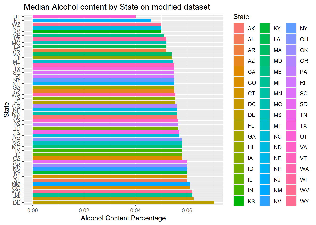
#Below is result of using complete data set with missing data to plot median of alcohol content
Beers.with.Breweries %>% group_by(State) %>%
  summarize(median_ABV=median(ABV),median_IBU=median(IBU))%>% ggplot()+
  geom_bar(mapping=aes(x=reorder(State,-median_ABV),y=median_ABV,fill=State),stat="identity")+
  coord_flip()+
  ggtitle("Median Alcohol content by State on non-Modified dataset")+xlab("State")+ylab("Alcohol Content Percentage")
## `summarise()` ungrouping output (override with `.groups` argument)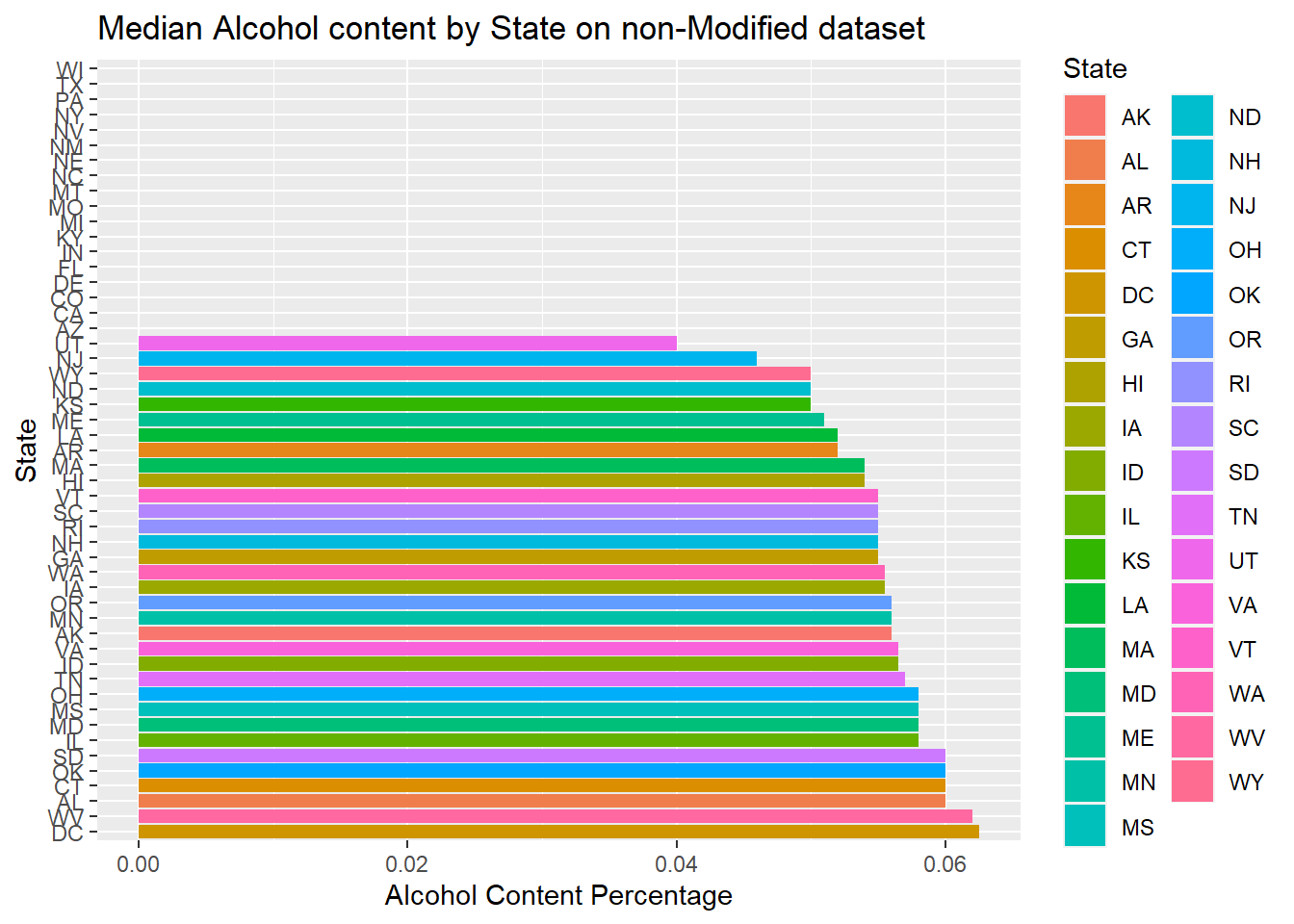
#Below is result of plotting median international bitterness unit for each state on modified data set
median %>% ggplot()+
  geom_bar(mapping=aes(x=reorder(State,-median_IBU),y=median_IBU,fill=State),stat="identity") +
  coord_flip()+
  ggtitle("Median International Bitterness Unit by State on modified dataset")+xlab("State")+ylab("International Bitterness Unit")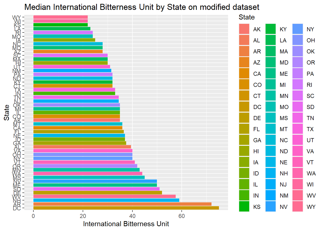
#Below is result of using complete data set with missing data to plot median of alcohol content
Beers.with.Breweries %>% group_by(State) %>%
  summarize(median_ABV=median(ABV),median_IBU=median(IBU))%>% ggplot()+
  geom_bar(mapping=aes(x=reorder(State,-median_IBU),y=median_IBU,fill=State),stat="identity") +
  coord_flip()+
  ggtitle("Median International Bitterness Unit by State on non-modified dataset")+xlab("State")+ylab("International Bitterness Unit")
## `summarise()` ungrouping output (override with `.groups` argument)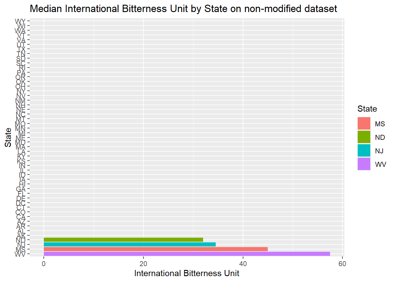
Exploring which state has the maximum alcoholic (ABV) beer and which state has the most bitter (IBU) beer
- As we can see below, Colorado ‘CO’ has the maximum alcoholic(ABV) beer, it is (0.128)
- This above result remain unchanged with the original data set
- As we can see, Oregon and Michigan have the most bitter beer
- Only Oregon has the most bitter beer in the unchanged data set. It means the Michigan beer bitterness value was imputed
# Discover which state has the maximum alcoholic beer
head(completedData %>%
  arrange(desc(ABV)) %>%
  select(State,ABV,Beer_Name))
## State ABV Beer_Name
## 1 CO 0.128 Lee Hill Series Vol. 5 - Belgian Style Quadrupel Ale
## 2 KY 0.125 London Balling
## 3 IN 0.120 Csar
## 4 CO 0.104 Lee Hill Series Vol. 4 - Manhattan Style Rye Ale
## 5 NY 0.100 4Beans
## 6 CA 0.099 Lower De Boom# Boxplot
completedData %>% ggplot(aes(x=ABV)) +
geom_boxplot(fill="green",outlier.colour="red", outlier.shape=8,
outlier.size=4, width=0.1) +
ggtitle("Boxplot showing distribution of ABV values")+xlab("Alcohol by volume")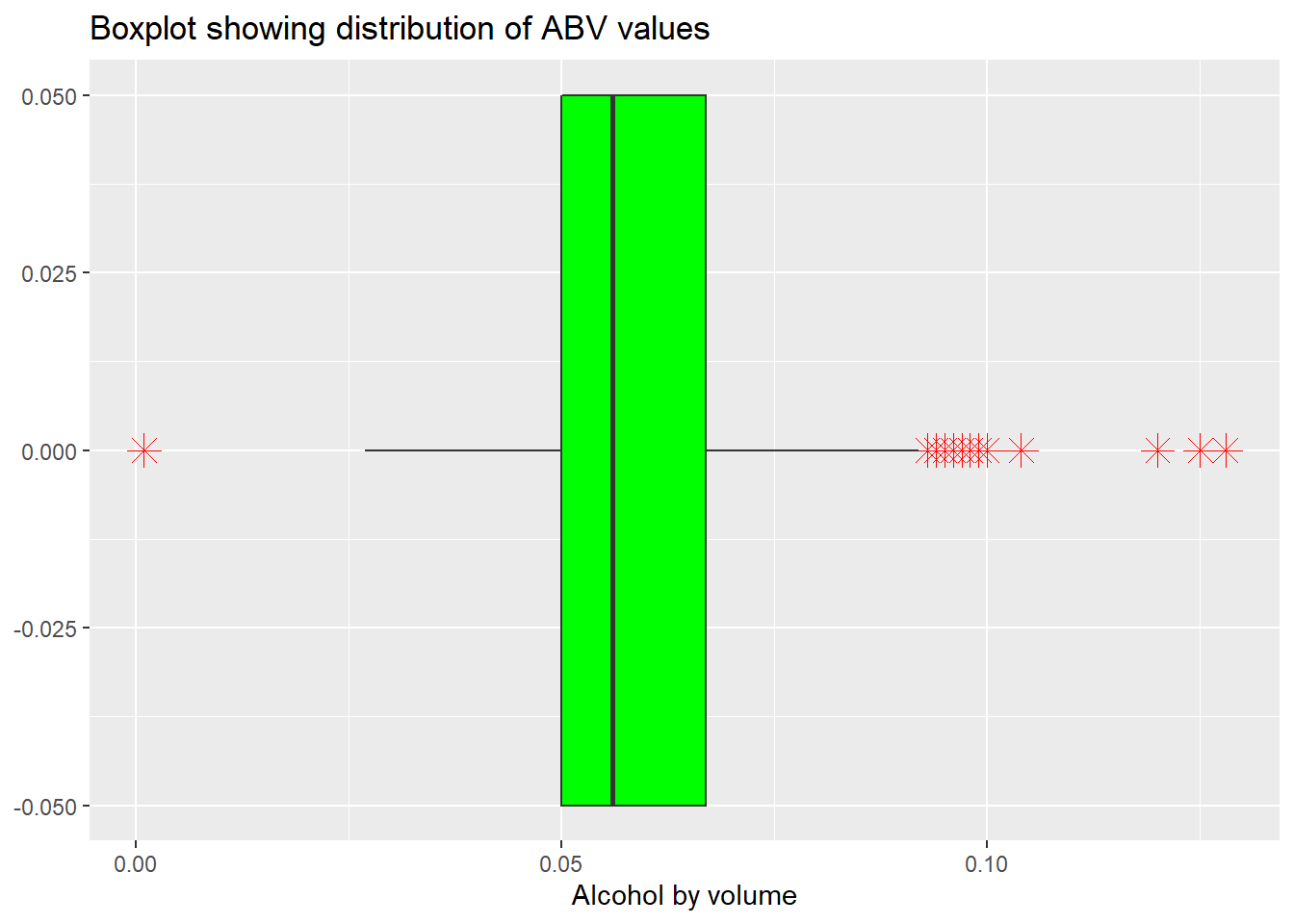
# Discover with un-changed data set
head(Beers.with.Breweries %>%
  arrange(desc(ABV)) %>%
  select(State,ABV,Beer_Name))
## State ABV Beer_Name
## 1 CO 0.128 Lee Hill Series Vol. 5 - Belgian Style Quadrupel Ale
## 2 KY 0.125 London Balling
## 3 IN 0.120 Csar
## 4 CO 0.104 Lee Hill Series Vol. 4 - Manhattan Style Rye Ale
## 5 NY 0.100 4Beans
## 6 CA 0.099 Lower De Boom# Discover which state has the most bitter (IBU) beer
head(completedData %>%
arrange(desc(IBU)) %>%
select(State,IBU,Beer_Name))## State IBU Beer_Name
## 1 OR 138 Bitter Bitch Imperial IPA
## 2 MI 138 Zaison
## 3 MI 138 Lemon Shandy Tripel
## 4 VA 135 Troopers Alley IPA
## 5 MI 130 Escoffier Bretta Ale
## 6 MA 130 Dead-Eye DIPA# Discover with un-changed data set
head(Beers.with.Breweries %>%
arrange(desc(IBU)) %>%
select(State,IBU,Beer_Name))## State IBU Beer_Name
## 1 OR 138 Bitter Bitch Imperial IPA
## 2 VA 135 Troopers Alley IPA
## 3 MA 130 Dead-Eye DIPA
## 4 OH 126 Bay of Bengal Double IPA (2014)
## 5 MN 120 Abrasive Ale
## 6 VT 120 Heady TopperIs there an apparent relationship between the bitterness of the beer and its alcoholic content?
- We can see from the scatter plot, there seem to be some sort of relationship between the two
- As ABV value increases, IBU seem to also increase
- This relationship seem to persist when we compare to the unmodified data
#first explore modified data
completedData %>%
  ggplot(aes(x=ABV, y=IBU)) +
  geom_point(size=2, shape=23, color = "dark green",position="jitter") +
  geom_smooth(method=lm) +
  ggtitle("IBU vs. ABV")+xlab("Alcohol by volume")+ylab("International Bitterness Unit")
## `geom_smooth()` using formula 'y ~ x'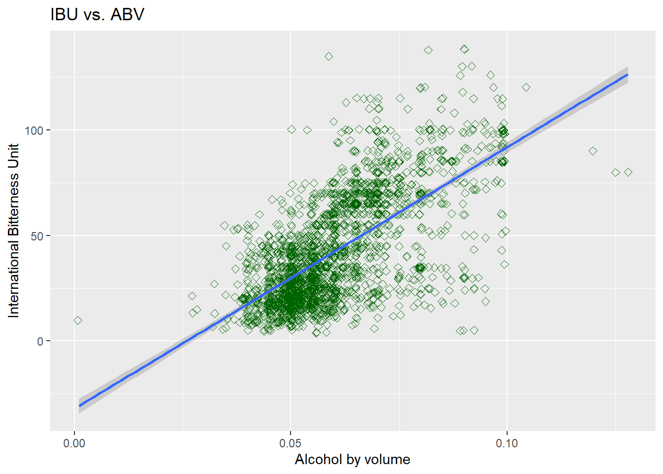
#next explore unmodified data
Beers.with.Breweries %>% select(ABV, IBU, State) %>%
  ggplot(aes(x=ABV, y=IBU)) +
  geom_point(size=2, shape=23, color = "dark green",position="jitter") +
  geom_smooth(method=lm) +
  ggtitle("IBU vs. ABV")+xlab("Alcohol by volume")+ylab("International Bitterness Unit")
## `geom_smooth()` using formula 'y ~ x'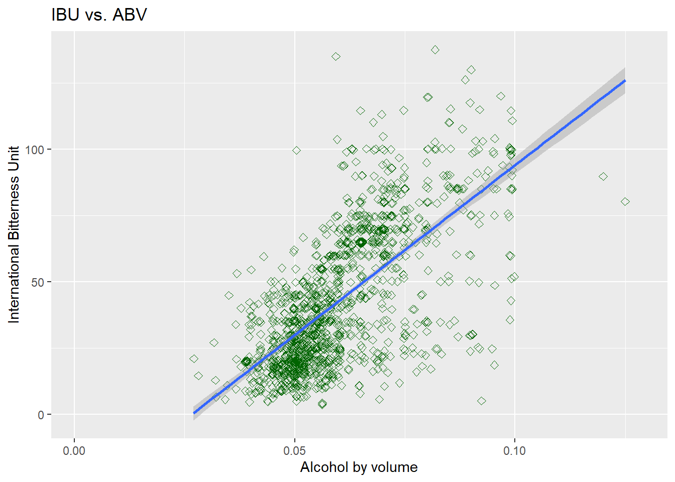
Budweiser would also like to investigate the difference with respect to IBU and ABV between IPAs (India Pale Ales) and other types of Ale (any beer with “Ale” in its name other than IPA).
- There are total of 954 Beer name has Ale or IPA in it
- 377 Beer name has India Pale Ales or IPA in it
- 577 are other types of Ale
- By using KNN model to try classifying India Pale Ales against other Ales
- Initially try k=5 (five neighbors to compare): Accuracy rate 0.79, sensitivity rate 0.65, Specificity rate 0.87
- Then we explored what is the best k value to give the most accuracy, after exploring average of 500 random sample, k=9 is about the best accuracy rate given
- Since Sensitivity is lowest among all, curious what is the best k for a good sensitivity rate?
- By running such test, it suggest k>37 provides a better Sensitivity rate, and not sacrificing accuracy rate too much (So to balance our model, we choose k=45 and rerun the test)
- In this scenario, we consider k=45 might be the best compromise to balance the model
- Getting an average result of one hundred random generations from KNN model with k=45, Average Accuracy = 0.80, Average Sensitivity = 0.78, Average Specificity = 0.81
- Conclusion: By tuning the model between accuracy and sensitivity (specificity is already pretty good), we decided to use k=45 for our KNN model and got average rate of successfully predicting India Pale Ales of 0.78, Average rate of successfully predicting Other types of Ales at 0.81, and overall average accuracy rate at 0.80.
- Next try Naive Bayes Models to use probabilities to estimate different Ales based on IBU and ABV
- After trying Naive Bayes Model with one random sample, Accuracy = 0.80, Sensitivity = 0.73, Specificity= 0.84
- By getting the average of one hundred random generations from NB model, Average Accuracy = 0.78, Average Sensitivity= 0.68, Average Specificity = 0.85
- Conclusion with NB model - almost as good as KNN k=9 prediction model, but depending on what is more important to client, such as, is it more important to predict other ales accurately, predicting IPA accurately or overall accuracy is most important
#In order to investigate the difference respect to IBU and ABV, first extract all name with Ales
#getting all bear name with ale in it (ignore the case factor)
all_ales = completedData %>% filter(str_detect(completedData$Beer_Name,regex("Ale|IPA",ignore.case=TRUE)))
india_pale_ales = all_ales %>%
  filter(str_detect(all_ales$Beer_Name,regex("India Pale Ale|IPA",ignore.case=TRUE)))
other_ales = all_ales %>%
  filter(!str_detect(all_ales$Beer_Name,regex("India Pale Ale|IPA",ignore.case=TRUE)))
# in order to effectively use KNN model, I decided to standardize percentage scale of ABV and IBU, so the effect of distance from ABV and IBU are roughly the same. I choose to use scale method to do so
all_ales$ABV = scale(all_ales$ABV)
all_ales$IBU = scale(all_ales$IBU)
# Change other ales name to other ales in order to use KNN model to test whether we can use IBU and ABV to distinguish IPAs from others
all_ales = all_ales %>%
  mutate(India.Pale.Ale.Or.Else = ifelse(str_detect(Beer_Name,regex("India Pale Ale|IPA",ignore.case=TRUE)),"India Pale Ale","Other Ale"))
#all_ales$India.Pale.Ale.Or.Else
# Start KNN test to see how good it is to use ABV and IBU to distinguish the Ales
library(class)
library(caret)
## Loading required package: lattice##
## Attaching package: 'caret'## The following object is masked from 'package:purrr':
##
## liftlibrary(e1071)
all_ales$India.Pale.Ale.Or.Else = as.factor(all_ales$India.Pale.Ale.Or.Else)
#Keep my result reproducible initially tried set.seed(100), try k=5
set.seed(101)
splitPerc = 0.8
trainIndices = sample(1:dim(all_ales)[1],round(splitPerc * dim(all_ales)[1]))
train = all_ales[trainIndices,]
test = all_ales[-trainIndices,]
# try k=5
classifications = knn(train[,3:4],test[,3:4],train$India.Pale.Ale.Or.Else, prob = TRUE, k = 5)
table(classifications,test$India.Pale.Ale.Or.Else)##
## classifications India Pale Ale Other Ale
## India Pale Ale 48 15
## Other Ale 26 102cm = confusionMatrix(table(classifications,test$India.Pale.Ale.Or.Else))
cm## Confusion Matrix and Statistics
##
##
## classifications  India Pale Ale Other Ale
##   India Pale Ale             48        15
##   Other Ale                  26       102
##
## Accuracy : 0.7853
## 95% CI : (0.7203, 0.8413)
## No Information Rate : 0.6126
## P-Value [Acc > NIR] : 2.578e-07
##
## Kappa : 0.5351
##
## Mcnemar's Test P-Value : 0.1183
##
## Sensitivity : 0.6486
## Specificity : 0.8718
## Pos Pred Value : 0.7619
## Neg Pred Value : 0.7969
## Prevalence : 0.3874
## Detection Rate : 0.2513
## Detection Prevalence : 0.3298
## Balanced Accuracy : 0.7602
##
## 'Positive' Class : India Pale Ale
## # explore best possible K value for accuracy
set.seed(101)
iterations = 500
numks = 50
masterAcc = matrix(nrow = iterations, ncol = numks)
for(j in 1:iterations)
{
trainIndices = sample(1:dim(all_ales)[1],round(splitPerc * dim(all_ales)[1]))
train = all_ales[trainIndices,]
test = all_ales[-trainIndices,]
for(i in 1:numks)
{
classifications = knn(train[,3:4],test[,3:4],train$India.Pale.Ale.Or.Else, prob = TRUE, k = i)
table(classifications,test$India.Pale.Ale.Or.Else)
CM = confusionMatrix(table(classifications,test$India.Pale.Ale.Or.Else))
masterAcc[j,i] = CM$overall[1]
}
}
MeanAcc = colMeans(masterAcc)
plot(seq(1,numks,1),MeanAcc, type = "l",main="mean Accuracy vs. different K (number of neighbor used to predict)",
ylab="Mean Accuracy",xlab="k used")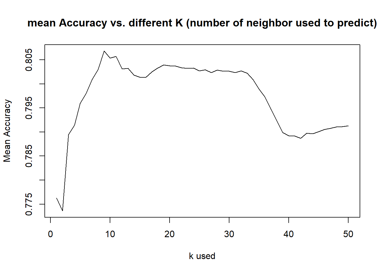
# explore best possible K value for sensitivity
set.seed(101)
iterations = 500
numks = 50
masterSen = matrix(nrow = iterations, ncol = numks)

for(j in 1:iterations)
{
trainIndices = sample(1:dim(all_ales)[1],round(splitPerc * dim(all_ales)[1]))
train = all_ales[trainIndices,]
test = all_ales[-trainIndices,]
for(i in 1:numks)
{
  classifications = knn(train[,3:4],test[,3:4],train$India.Pale.Ale.Or.Else, prob = TRUE, k = i)
  table(classifications,test$India.Pale.Ale.Or.Else)
  CM = confusionMatrix(table(classifications,test$India.Pale.Ale.Or.Else))
  masterSen[j,i] = CM$byClass[1]
}
}
MeanSen = colMeans(masterSen)
plot(seq(1,numks,1),MeanSen, type = "l",main="mean Sensitivity vs. different K (number of neighbor used to predict)",
     ylab="Mean Sensitivity",xlab="k used")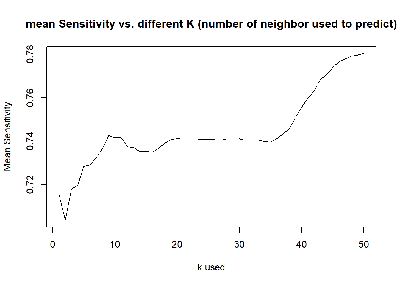
#Get an average percentage of Accuracy, Sensitivity, and Specificity of KNN model k=45
set.seed(101)
iterations = 100
numks = 50
masterAcc = matrix(nrow = iterations, ncol = 1)
masterSen = matrix(nrow = iterations, ncol = 1)
masterSpec = matrix(nrow = iterations, ncol = 1)
for(j in 1:iterations)
{
trainIndices = sample(1:dim(all_ales)[1],round(splitPerc * dim(all_ales)[1]))
train = all_ales[trainIndices,]
test = all_ales[-trainIndices,]
classifications = knn(train[,3:4],test[,3:4],train$India.Pale.Ale.Or.Else, prob = TRUE, k = 45)
CM = confusionMatrix(table(classifications,test$India.Pale.Ale.Or.Else))
masterAcc[j,1]=CM$overall[1]
masterSen[j,1]=CM$byClass[1]
masterSpec[j,1]=CM$byClass[2]
}
MeanAcc = colMeans(masterAcc)
MeanSen = colMeans(masterSen)
MeanSpec = colMeans(masterSpec)
MeanAcc
## [1] 0.7978534MeanSen## [1] 0.7759099MeanSpec## [1] 0.812105# Try using Naive Bayes see if it will improve results, split 0.8:
set.seed(102)
splitPerc = 0.8
trainIndices = sample(1:dim(all_ales)[1],round(splitPerc * dim(all_ales)[1]))
train = all_ales[trainIndices,]
test = all_ales[-trainIndices,]
#NB model
model = naiveBayes(train[,3:4],train$India.Pale.Ale.Or.Else)
CM = confusionMatrix(table(predict(model,test[,3:4]),test$India.Pale.Ale.Or.Else))
CM## Confusion Matrix and Statistics
##
##
## India Pale Ale Other Ale
## India Pale Ale 57 18
## Other Ale 21 95
##
## Accuracy : 0.7958
## 95% CI : (0.7316, 0.8506)
## No Information Rate : 0.5916
## P-Value [Acc > NIR] : 1.65e-09
##
## Kappa : 0.5749
##
## Mcnemar's Test P-Value : 0.7488
##
## Sensitivity : 0.7308
## Specificity : 0.8407
## Pos Pred Value : 0.7600
## Neg Pred Value : 0.8190
## Prevalence : 0.4084
## Detection Rate : 0.2984
## Detection Prevalence : 0.3927
## Balanced Accuracy : 0.7857
##
## 'Positive' Class : India Pale Ale
## # Try getting average of Accuracy, Sensitivity and Specificity rate using NB model from 100 random generators
set.seed(101)
splitPerc = .8
iterations = 100
masterAcc = matrix(nrow = iterations, ncol = 1)
masterSen = matrix(nrow = iterations, ncol = 1)
masterSpec = matrix(nrow = iterations, ncol = 1)
for(j in 1:iterations)
{
trainIndices = sample(1:dim(all_ales)[1],round(splitPerc * dim(all_ales)[1]))
train = all_ales[trainIndices,]
test = all_ales[-trainIndices,]
#NB model
model = naiveBayes(train[,3:4],train$India.Pale.Ale.Or.Else)
CM = confusionMatrix(table(predict(model,test[,3:4]),test$India.Pale.Ale.Or.Else))
masterAcc[j,1]=CM$overall[1]
masterSen[j,1]=CM$byClass[1]
masterSpec[j,1]=CM$byClass[2]
}
MeanAcc = colMeans(masterAcc)
MeanSen = colMeans(masterSen)
MeanSpec = colMeans(masterSpec)
MeanAcc## [1] 0.7837173MeanSen## [1] 0.6808075MeanSpec## [1] 0.8485147Further exploration – Free Style
- Explore Types of Ales produced in each city (Which cities contribute to most varieties of Ales?)
- Explore all bear counts by city
- Explore average ABV content produced by state (Which states produces higher average ABV content, which states lower?)
- Note: Since map_data library don’t have Hawaii and Alaska map data to plot, that’s why it is not showing on the map, even we have a few breweries in those states.
Density of Ales count by city
#import map library
library(maps)
##
## Attaching package: 'maps'## The following object is masked from 'package:purrr':
##
## maplibrary(plotly)##
## Attaching package: 'plotly'## The following object is masked from 'package:ggplot2':
##
## last_plot## The following object is masked from 'package:stats':
##
## filter## The following object is masked from 'package:graphics':
##
## layout# Import US Cities location data
uscities <- read.csv("/Users/ysojd/Desktop/GRAD SCHOOL COURSEWORK/MSDS_6306_Doing-Data-Science-Master/MSDS_6306_Doing-Data-Science-Master/Case Study 1/uscities.csv",header = TRUE)
uscities = uscities%>%rename(City = city)
uscities = uscities%>% group_by(City) %>% filter(row_number()==1)
#Loading in State Coordinates
state_coord <- read.csv("/Users/ysojd/Desktop/GRAD SCHOOL COURSEWORK/MSDS_6306_Doing-Data-Science-Master/MSDS_6306_Doing-Data-Science-Master/Case Study 1/MSDS6306-Case-Study1-master/states_coord.csv",header = TRUE)
# Getting all Ales Beer available
allAles2 = completedData %>% filter(str_detect(completedData$Beer_Name,regex("Ale",ignore.case=TRUE)))
dataWithMap = left_join(allAles2,uscities, by = "City")
#str(dataWithMap)
#dataWithMap %>% filter((is.na(lng))|(is.na(lat))) %>% select(Brew_Name,City)
dataWithMap2 = dataWithMap %>% select(Beer_Name,City,lat,lng,state)
#head(dataWithMap2,100)
dataWithMap3 = dataWithMap2 %>% group_by(City) %>% mutate(count = n())
dataWithMap3 = dataWithMap3 %>% group_by(City)%>%filter(row_number()==1)%>%
filter((!is.na(lng))&(!is.na(lat)))
states <- map_data("state")
p <- ggplot() +
geom_polygon(data = states, aes(x = long, y = lat, group = group), fill = "yellow", color = "black") +
coord_quickmap()
p <-p + geom_point(data = dataWithMap3, aes(x = lng, y = lat, size=count,alpha=count),color="blue")+
geom_text(data = state_coord, aes(x = longitude, y = latitude, label = state))+
ggtitle("Density of Ales count by City") + xlab("Longitude")+ylab("Latitute")
ggplotly(p)All Beer types count by City
# Getting all Beer available
dataWithMap = left_join(completedData,uscities, by = "City")
#str(dataWithMap)
#dataWithMap %>% filter((is.na(lng))|(is.na(lat))) %>% select(Brew_Name,City)
dataWithMap2 = dataWithMap %>% select(Beer_Name,City,lat,lng,state)
#head(dataWithMap2,100)
dataWithMap3 = dataWithMap2 %>% group_by(City) %>% mutate(count = n())
dataWithMap3 = dataWithMap3 %>% group_by(City)%>%filter(row_number()==1)%>%
  filter((!is.na(lng))&(!is.na(lat)))
states <- map_data("state")
p <- ggplot() +
  geom_polygon(data = states, aes(x = long, y = lat, group = group), fill = "yellow", color = "black") +
  coord_quickmap()

p <-p + geom_point(data = dataWithMap3, aes(x = lng, y = lat, size=count,alpha=count),color="blue")+
  geom_text(data = state_coord, aes(x = longitude, y = latitude, label = state))+
  ggtitle("Density of all Beer count by City") + xlab("Longitude")+ylab("Latitute")
ggplotly(p)
Average ABV Heatmap (by state)
library(ggplot2)
library(dplyr)
library(mapproj)
library(plyr)
## ------------------------------------------------------------------------------## You have loaded plyr after dplyr - this is likely to cause problems.
## If you need functions from both plyr and dplyr, please load plyr first, then dplyr:
## library(plyr); library(dplyr)## ------------------------------------------------------------------------------##
## Attaching package: 'plyr'## The following objects are masked from 'package:plotly':
##
## arrange, mutate, rename, summarise## The following object is masked from 'package:maps':
##
## ozone## The following object is masked from 'package:purrr':
##
## compact## The following objects are masked from 'package:dplyr':
##
## arrange, count, desc, failwith, id, mutate, rename, summarise,
## summarizelookup = data.frame(abb = state.abb, State = state.name) #makes a data frame with State name and abbreviation.
#lookup
colnames(completedData)[10] = "abb"
completedData$abb = as.character(completedData$abb)
Breweries2 = merge(completedData,lookup, by.x = "abb", by.y="abb", all.x=TRUE) # make one dataset with state names and abb
#Breweries2
Breweries2$ABV <- as.numeric(Breweries2$ABV)
BreweriesMapData <- Breweries2 %>% select(ABV, State) %>% group_by(State)
#BreweriesMapData
BreweriesMapData <- aggregate(. ~ State, BreweriesMapData, mean)
BreweriesMapData$region <- tolower(BreweriesMapData$State)
BreweriesMapData = BreweriesMapData[-1]
#BreweriesMapData
states <- map_data("state")
#states
map.df <- full_join(states,BreweriesMapData, by="region", all.x=T)
#map.df
map.df <- map.df[order(map.df$order),]
h <- ggplot(map.df, aes(x=long,y=lat))+
geom_polygon(aes(fill=ABV))+
geom_path(aes(group=group))+
geom_text(data = state_coord, aes(x = longitude, y = latitude, label = state))+
scale_fill_gradientn(colours=rev(heat.colors(5)),na.value="grey90")+ggtitle("Average ABV By State")+
coord_map()
ggplotly(h)
Comment on the summary statistics and distribution of the ABV variable.